Choosing the Correct Test Target

Components of Image Quality | Depth of Field | Types of Test Targets | Application Examples

Test targets are useful when evaluating or calibrating an imaging system's performance or image quality. This could include troubleshooting the system, certifying or evaluating measurements, as well as establishing a foundation to ensure the system works well with another. Image quality can be defined by different components, particularly resolution, contrast, modulation transfer function (MTF), depth of field (DOF), and distortion; therefore, one or more types of test targets may be necessary or helpful depending upon the type of system being constructed or what needs to be measured. Fortunately, an array of targets exists that cater towards specific systems including cameras, visual displays, or even a single, thin lens. To be able to choose the correct test target, it is important to first understand the components of image quality.

COMPONENTS OF IMAGE QUALITY

Resolution

Resolution is an imaging system's ability to distinguish object detail. It is often expressed in terms of line-pairs per millimeter (lp/mm) as seen in Figure 1. A low resolution image usually lacks fine detail and is often blurry, whereas a high resolution image is highly detailed and clear.

Figure 1: Relation of Line-Pairs to Square Waves

To illustrate this concept, imagine two squares being imaged onto pixels of a CCD camera. Assuming that the primary magnification of the lens is such that one square fills one camera pixel (Figure 2a), if there is no space between the filled pixels, it will appear as one large, red rectangle. However, if "white space", or space distinctively different from the original pixel color, is found between the pixels, the camera will be able to distinguish among the two squares (Figure 2b). Hence, the pairing of the red square and "white space" becomes one lp/mm, which corresponds to two separate pixels.

Pair of Red Squares Unresolved vs. Resolved

Figure 2: Pair of Red Squares Unresolved (a) vs. Resolved (b)

Contrast

Contrast is a measurement of the separation between the light and dark regions of an image. More specifically, contrast is a change in the intensity or brightness from one point to another. It affects how effectively the differences between the object and the shades of gray in the background are reproduced. An image with the highest contrast is one in which black is truly black and white is truly white, without any shades of gray in between. As contrast is reduced, the distinction between black and white begins to blur, in a very literal sense, and shades of gray appear (Figure 3).

Figure 3: Contrast in Relation to Pixels

Contrast is often expressed in terms of percentage (%) and is calculated by using Maximum Intensity (I_max) and Minimum Intensity (I_min), as expressed in Equation 1. It can also be represented by a periodic function (i.e. square wave or sine wave), or a function that alternates regularly and instantaneously between two levels.

(1)$$ \text{% Contrast} = \left[ \frac{I_{\text{max}} - I_{\text{min}}}{I_{\text{max}} + I_{\text{min}}} \right] $$

Modulation Transfer Function (MTF)

Modulation Transfer Function, or MTF, is a measurement of an imaging lens' ability to transfer contrast from the object plane to the image plane at a specific resolution. The object and image planes are the spatial areas where the object and the image preside. The object plane is in front of the imaging system, and the image plane is either in front or behind the imaging system depending on whether the image is real or virtual. MTF is expressed with respect to image resolution (lp/mm) and contrast (%), as seen in Figure 4. Typically, as resolution increases, contrast decreases until a cut-off point, at which the image becomes irresolvable and grey.

Figure 4: Example MTF Curve of 0.13X PMAG Imaging Lens

Another component of MTF, in addition to the aforementioned resolution and contrast, is diffraction limit. Diffraction limit is a physical limit restricting a lens from being able to image points or edges perfectly. Since it is constrained by the wave nature of light, even a "perfectly" designed and manufactured lens cannot achieve diffraction limited performance. However, designers utilize a variety of methods to reduce aberrations and increase overall system accuracy in order to come as close as possible to reaching a system's ideal diffraction limit.

Correspondingly, a len's geometry contributes to its ability to reproduce good quality image. Lens Diameter (D), Focal Length (f) and f/# (Equation 2) all affect MTF.

(2)$$ f/ \# = \frac{f}{D} $$

f/# is the light gathering ability of a lens. As Lens Diameter increases, f/# decreases. Low f/# lenses collect the most light, thereby making them ideal for light restrictive applications. Although high f/# can improve an imaging lens' performance, increasing it too much can be detrimental because it can cause the diffraction limit to become progressively worse.

Depth of Field (DOF)

Depth of Field, or DOF, is the ability of a lens to maintain a desired amount of image quality as the object being viewed moves in and out of focus. DOF is defined with an associated resolution and contrast, as both suffer when an object is placed closer or farther from the optimal working distance (Figure 5). DOF also applies to objects with depth, since high DOF lenses can image the whole object clearly. DOF is estimated by a single value calculated from the diffraction limit, making it a theoretical approximation. It is difficult, however, to make a genuine comparison because many imaging lenses are not diffraction limited. For example, two lenses may have the same f/# (i.e. equal diffraction limit), but do not necessarily have similar performance or comparable DOF. Therefore, the only way to truly determine DOF is to use a test target to test it.

Figure 5: Geometric Representation of DOF for Low and High f/# Imaging Lenses

Distortion

Distortion is a type of geometrical aberration that causes a difference in magnification of the object at different points in the image. As light rays carry the image of an object through a system, various points are misplaced relative to the center of the field, or the central point of the image. Therefore, distortion is not an aberration that causes blurs, but an aberration that causes a dislocation. Distortion is calculated by:

(3)$$ \text{% Distortion} = \left( \frac{\text{AD} - \text{PD}}{\text{PD}} \right) \times 100 \% $$

where AD is the Actual Distance and PD is the Paraxial, or Predicted, Distance.

Distortion, represented by a percentage, can be either positive or negative. A positive percentage represents "pincushion" distortion, whereas a negative percentage represents "barrel" distortion. Figure 6 illustrates barrel and pincushion distortion compared to an ideal, perfectly square non-distorted image.

Figure 6: Barrel and Pincushion Distortion

Although distortion is present in almost all lenses, it can be corrected by using short focal lengths. Unfortunately, short focal length systems tend to suffer from more diffraction effects than their longer focal length counterparts. Correcting for one component of image quality undeniably affects another, a fact that must always be taken into account. An important concept to keep in mind is that distortion causes information about the object to be misplaced but not lost. The original, un-distorted image can be reconstructed through image analysis software.

TYPES OF TEST TARGETS

A variety of test targets exist to help characterize resolution, contrast, modulation transfer function (MTF), depth of field (DOF), and distortion in an imaging system. Use the following guide of the most popular targets to make choosing the correct test target as easy as possible.

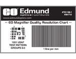
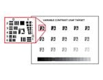
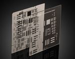
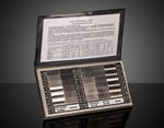
1951 USAF Resolution Targets
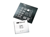Consist of horizontal and vertical bars organized in groups and elements. Each group is comprised of up to nine elements within a range of twelve groups. Every element is composed of three horizontal and three vertical bars equally spaced with one another within a group and corresponds to an associated resolution based on bar width and space. The vertical bars are used to calculate horizontal resolution and horizontal bars are used to calculate vertical resolution. These targets are very popular when considering a target for testing resolution. View Product
Typical Applications
Testing Resolution in Applications such as Optical Test Equipment, Microscopes, High Magnification Video Lenses, Fluorescence and Confocal Microscopy, Photolithography, and Nanotechnology

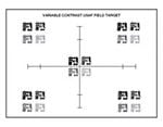
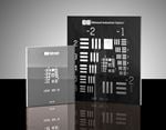
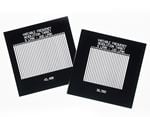
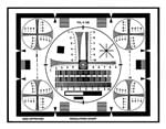
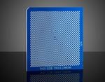
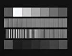
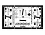
IEEE Resolution Targets
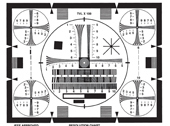Designed to characterize the amount of resolution a camera or display system is able to reproduce from an original image. Because resolution can be different throughout the field of view, both horizontal and vertical resolution can be measured in the center of the target as well as the four corners. IEEE Resolution Targets can also be used to check scanning, linearity, aspect, shading, and interlacing, as well as measure TV lines. View Product
Typical Applications
Testing of Analog Imaging Systems

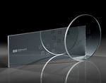
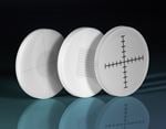
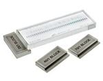
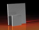
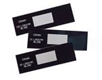
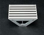
Ronchi Rulings
Consist of a square wave optic with constant bar and space patterns that carry a high contrast ratio. They are ideal for reticle and field calibration requirements, and often used for evaluating resolution, field distortion and parafocal stability. Ronchi Rulings are not limited to only calculating resolution; they can be used for diffraction testing. View Product
Typical Applications
Testing the Parameters of Resolution and Contrast, Diffraction Testing

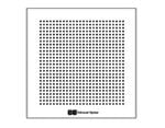
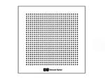
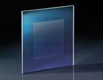
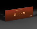
Distortion Targets
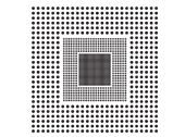Used for calibrating imaging systems for distortion, which is a geometrical aberration that may misplace certain parts of the image. These targets consist of a grid of dots that are separated by various distances depending on the application. View Product
Typical Applications
Lower Focal Length Lenses, Systems that Carry a Wide Field of View

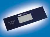
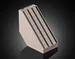
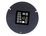
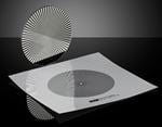
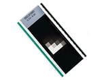
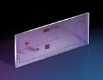
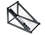
Depths of Field Targets
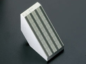Directly test the depth of field in imaging systems without the use of calculations. The target should be mounted 45° from the face of the lens that is parallel to the object to be viewed; the scale of the target consists of horizontal and vertical lines that measure frequency in line pairs per mm (lp/mm). View Product
Typical Applications
Circuit Board Inspection, Security Cameras

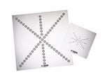
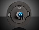
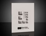
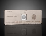
Star Targets
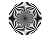Ideal for identifying focus errors, astigmatism, as well as other focus differing aberrations. The target consists of a circle formed with alternating black and white radial lines emanating from a central point. Because the lines taper, a continuous change in resolution is present and can be measured in both vertical and horizontal directions without repositioning. View Product
Typical Applications
Alignment of a System, Assistance with Assembly, Comparing Highly Resolved or Magnified Imaging Systems

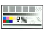
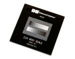
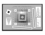
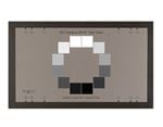
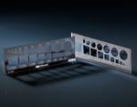
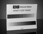
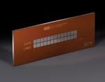
EIA Grayscale Targets
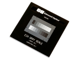Useful for testing optical and video inspection systems, and consist of a standard pattern and carry two scales, one linear and the other logarithmic, which is useful depending on the linearity of the detector being used. Each scale has nine steps that are acutely tuned for a precise halftone pattern. View Product
Typical Applications
Optical and Video Inspection Systems, Evaluating Contrast Levels in Cameras

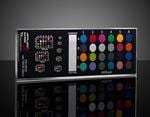
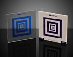
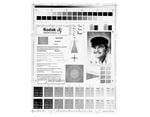
Color Checker Targets
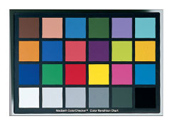Used to determine true color balance or optical density of any color rendition system. They may be expanded to include more squares with a different assortment of colors and act as a reference for testing and standardizing color inspection and analysis systems. View Product
Typical Applications
Color Rendition Systems, Digital Cameras and Photography

Exploring 1951 USAF Resolution Targets

1951 USAF Resolution Targets have been and are currently a standard when considering a target that tests the resolution of an imaging system. They consist of horizontal and vertical bars organized in groups and elements. Each group is composed of six elements, and each element is composed of three horizontal and three vertical bars equally spaced with one another. There can be a total of twelve groups, with larger numbers used for higher resolution. For example, a standard resolution 1951 target consists of group numbers from -2 to 7, whereas a high resolution of -2 to 9; the element number is the same. The resolution is based on bar width and space, where the length of the bars is equal to five times the width of a bar (Figure 7). One Line Pair (lp) is equivalent to one black bar and one white bar. Vertical bars are used to calculate horizontal resolution and horizontal bars are used to calculate vertical resolution.

Figure 7: 1951 USAF Target Specifications

Qualitatively, the resolution of an imaging system is defined as the group and element combination directly before the black and white bars begin to blur together. Quantitatively, resolution (in terms of line pairs per millimeter, or lp/mm) can be calculated by:

(4)$$ \text{Resolution} = 2^ \left({\text{Group Number} \, + \, \frac{\text{Element Number} - 1}{6}}\right) $$

It is important to keep in mind that calculating resolution with a 1951 USAF Target is subjective. In other words, it depends on who is looking at the target. Someone with 20/20 vision (using the Snellen Ratio) is able to discern higher resolution than someone with, for example, 20/25 or 20/30 vision. Even though the actual test yields precise resolution values, the user's vision can lead to imprecise measurements.

APPLICATION EXAMPLES

Example 1: Calculating Resolution with a 1951 USAF Resolution Target

When given a specified group and element number, one can easily calculate the resolution in lp/mm using Equation 4. For instance, if the vertical or horizontal bars start to blur at group 4 element 3, the resolution of the system can be designated as group 4 element 2. To quickly calculate resolution, use our 1951 USAF Resolution EO Tech Tool.

(5) \begin{align} \text{Resolution} & = 2^ \left({\text{Group Number} \, + \, \frac{\text{Element Number} - 1}{6}}\right) \\ & = 2^\left({4 + \frac{2-1}{6}}\right) = 18 \tfrac{\text{lp}}{\text{mm}} \end{align}

To convert lp/mm to microns (μm), simply take the reciprocal of the lp/mm resolution value and multiply by 1000.

(6) \begin{align} \text{Resolution} \left[ \large{\unicode[arial]{x03BC}} \text{m} \right] & = \frac{1000 \tfrac{ \large{\unicode[arial]{x03BC}} \text{m}}{\text{mm}}}{\text{Resolution} \left[ \tfrac{\text{lp}}{\text{mm}} \right]} \\ & = \frac{1000 \tfrac{ \large{\unicode[arial]{x03BC}} \text{m}}{\text{mm}}}{18 \tfrac{\text{lp}}{\text{mm}}} = 55.5 \large{\unicode[arial]{x03BC}} \text{m} \end{align}

Example 2: Understanding f/#

To understand the relationship between f/#, depth of field, and resolution, consider an example with a 35mm Double Gauss Imaging Lens (Figure 8). In this example, the lens will be integrated into a system which requires a minimum of 5 lp/mm (200μm) object resolution at 20% contrast. The diffraction limit ξ_c, or cutoff frequency, is determined by Equation 7:

(7)$$ \xi_c = \frac{1}{\lambda \cdot \left( f/ \# \right)} $$

Graphical Representation of Resolution vs. f/# and DOF vs. f/#

Figure 8: Graphical Representation of Resolution vs. f/# (Left) and DOF vs. f/# (Right) for a 35mm Double Gauss Imaging Lens

where λ is the wavelength of the system. For simplicity, Equation 7 assumes a non-aberrated, ideal system. Because this system is expected to have aberrations, though, the diffraction limit decreases with increasing f/#. Determining an ideal f/# for this system leads to calculating the highest possible depth of field. Comparing resolution vs. f/#, it is evident that below f/3, the lens is limited by aberrations and cannot obtain the minimum desired resolution. However, "stopping down" or closing the iris reduces aberrations and improves DOF. At f/4.2, diffraction effects caused by the optical elements within the imaging lens become more prominent than the effects from aberrations; this is the point at which the lens becomes diffraction limited. Beyond f/4.2, closing the aperture increases DOF, but reduces resolution. At f/13.5, the diffraction limit defines the extent of the desired resolution. Beyond f/13.5, resolution continues to decrease while DOF continues to increase. In this particular example, f/13.5 is the ideal f/# for an optimum depth of field at a minimum resolution.